library(rvest)
library(tidyverse)
library(jsonlite)
library(janitor)
library(here)
source(here("data/helperCNNAnalysis.R"))Analyzing the CNN coverage of the Prague University shooting
This Article, while only analyzing the reporting about a mass shooting will still contain some references about it. Read with caution if you are sensitive to that.
Given that the University shooting that happened on the 21 December 2023 was unprecedented in Czech history, I wondered whether it would be reflected as such in american media that has grown increasingly desensitized to news of mass shootings.
Resources used
I used the web-scraping tutorial provided by renatatopinkova and the book Text Mining with R (Robinson and Silge 2024). ChatGPT-4 and its internal module R-Guru were used for troubleshooting.
Getting the data
I wanted to compare the mass shooting to comparable reporting about mass shootings using the same live-block format CNN used for the Prague shooting. I used the first 12 articles that popped up for the Google search ‘site:cnn.com “mass shooting” live-news’ and filtering for articles in 2023-2024.
I created a list of the necessary URLs and a couple of helper functions: readUrlList, parseUrlList and generateTeiCorpus. They are simple for-loops that do what their name suggest. Let’s load them together with the packages we will need.
Now we can use them to read and parse the HTML of the CNN live-blogs. This may take some time so lets save it for later. If the code should be broken I have provided my own webscrape from 28.02.2024.
htmlList <- readUrlList(urlList, silent = T)
parsedDt <- parseUrlList(htmlList, silent = T)
saveRDS(parsedDt, file = "data/parsedDt_WebscrapingCNN.rds")
parsedDt
Alternative:
parsedDt <- readRDS(here("data/parsedDt_WebscrapingCNN.rds"))
parsedDt
As we can see, we don’t really see the article text (the last column “liveBlogUpdate”) we need to un-nest the data and fix the column names while we are at it.
blogPostsExpanded <- parsedDt %>%
  unnest(cols = c(liveBlogUpdate), names_sep = "_blog") %>%
  rename_with(~ str_replace_all(.x, "[@\\$]", "")) %>%
  select(mainEntityOfPage:datePublished, author:liveBlogUpdate_blogheadline, liveBlogUpdate_blogauthor:liveBlogUpdate_blogarticleBody)

blogPostsExpanded
TEI conversion
Some tools require a TEI compatible corpus such as: https://voyant-tools.org/. We will now convert our data:
blogTEI <- blogPostsExpanded %>%
  mutate(
    MetadataColumn = paste0("eventName: ", about$name, "headline:", liveBlogUpdate_blogheadline),
    TextColumn = liveBlogUpdate_blogarticleBody
  )

description <- paste0("A TEI corpus containg ", length(blogTEI), " live blogpost from CNN about mass shootings.")

prague <- generateTeiCorpus(MetadataColumn = blogTEI$MetadataColumn, TextColumn = blogTEI$TextColumn, MetadataSting = description, silent = T)
Analysis in R
If we want to keep analyzing in R we have multiple options. I would refer you to the great book ‘Text Mining with R’. Let’s use the tidytext and textdata packages to do a simple sentiment analysis. First we need to shape our data accordingly.
library(tidytext)
library(textdata)

# Analysis
reducedTb <- blogPostsExpanded %>%
  unnest(cols = c(about)) %>%
  select(name, liveBlogUpdate_blogheadline, liveBlogUpdate_blogarticleBody) %>%
  rename("headline" = liveBlogUpdate_blogheadline, "text" = liveBlogUpdate_blogarticleBody) %>%
  mutate(
    text = tolower(text),
    name = gsub("April 10, 2023: |April 11, 2023 - |Live updates: |March 27, 2023 |May 3, 2023 - |October 25, 2023 - ", "", name),
    name = str_wrap(name, width = 40)
    ) %>%
  unnest_tokens(word, text) %>%
  anti_join(stop_words, by = "word")

NrcSentiments <- get_sentiments("nrc") # Get the sentiment database

# Join our webscraped date with the sentiment file
articlesSentiment <- reducedTb %>%
  inner_join(NrcSentiments, by = "word", relationship = "many-to-many") %>%
  count(name, sentiment) %>%
  pivot_wider(names_from = sentiment, values_from = n) %>%
  mutate(
    total = rowSums(select(., anger:trust)),
    other = rowSums(select(., c(disgust, joy, surprise))),
    reducedTb %>% group_by(name) %>% summarise(articles = n_distinct(headline)) %>% select("articles"), # Direct add articles
    across(anger:other, ~ .x / total, .names = "{.col}Prop")
  )

# Pivot into a long format for the purpose of plotting
articlesSentimentLong <- articlesSentiment %>%
  select(name, angerProp, anticipationProp, fearProp, negativeProp:sadnessProp, trustProp, otherProp) %>%
  pivot_longer(cols = angerProp:otherProp,  names_to = "emotion", values_to = "prevalence") %>%
  mutate(emotion = gsub("Prop", "", emotion))

unique(articlesSentimentLong$emotion)
[1] "anger" "anticipation" "fear" "negative" "positive"
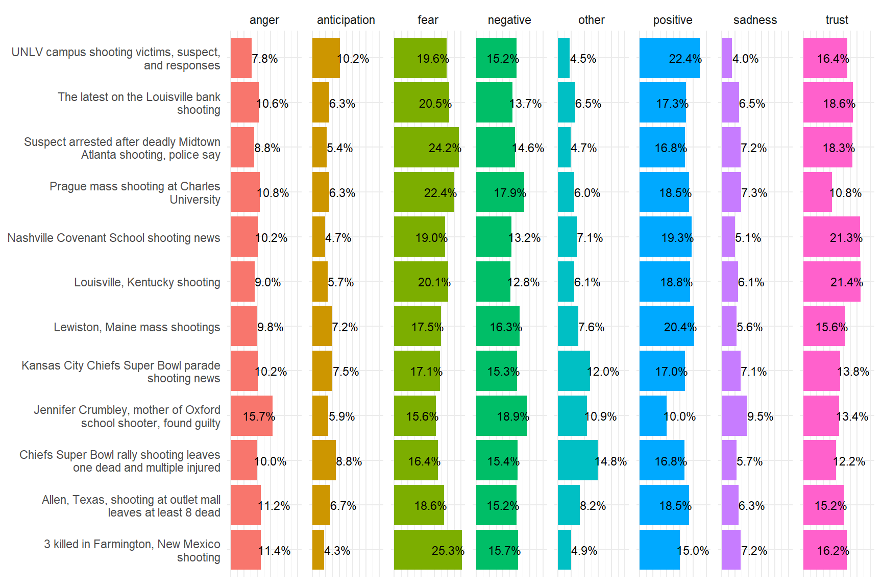
[6] "sadness" "trust" "other" We have reduced our data and joined it with the sentiment database nrc published by Saif Mohammad and Peter Turney. After that we computed rowSums and ‘rowAverages’, finally we converted the data into a long format for the purpose of plotting. For that we will be using the packages ggplot2 and scales.
library(ggplot2)
library(scales)
Attaching package: 'scales'The following object is masked from 'package:purrr':
discardThe following object is masked from 'package:readr':
col_factorggplot(articlesSentimentLong) +
aes(x = name, y = prevalence, fill = emotion) +
geom_col() +
geom_text(
aes(label = percent(prevalence, accuracy = 0.1)),
nudge_y = if_else(articlesSentimentLong$prevalence > .15, -.05, .05),
size = 3,
color = "black") +
coord_flip() +
theme_minimal() +
theme(axis.ticks = element_blank(),
axis.text.x = element_blank(),
axis.title.x = element_blank(),
axis.title.y = element_blank(),
legend.position = "none") +
facet_grid(~ emotion)
Expanding on that analysis: Latent Dirichlet allocation
Latent Dirichlet allocation (LDA) is a particularly popular method for fitting a topic model. It treats each document as a mixture of topics, and each topic as a mixture of words. We will use it to give some oomph to our analysis. For that we will be using the package topicmodels. We will also have to adapt the shape of our data:
library(topicmodels)

removeWords <- c("cnn", "p.m")
toRemoveDf <- tibble(document = NA, word = removeWords, n = 1)

# Dataformatting
# Need one-term-per-document-per-row

DtmData <- reducedTb %>%
  group_by(name, headline) %>%
  count(word, sort = T) %>%
  ungroup() %>%
  mutate(document = paste0(name, "_", headline)) %>%
  select(document, word, n) %>%
  anti_join(toRemoveDf, by = "word")

head(DtmData, 5)
Now that our data is in an appropriate format we can start modeling. As we know that there are 12 Events we have scraped from the Web we can input that for gaining an optimal model. (I have attempted other values, the results were less than stellar.)
castData <- cast_tdm(data = DtmData, term = document, document = word, value = n) # reverse necessary

castData
<<TermDocumentMatrix (terms: 432, documents: 3991)>>
Non-/sparse entries: 20266/1703846
Sparsity : 99%
Maximal term length: 180
Weighting : term frequency (tf)model1 <- LDA(castData, k = 12, control = list(seed = 1234)) # reverses, see above
model1A LDA_VEM topic model with 12 topics.model1Topics <- tidytext::tidy(model1, matrix = "beta")
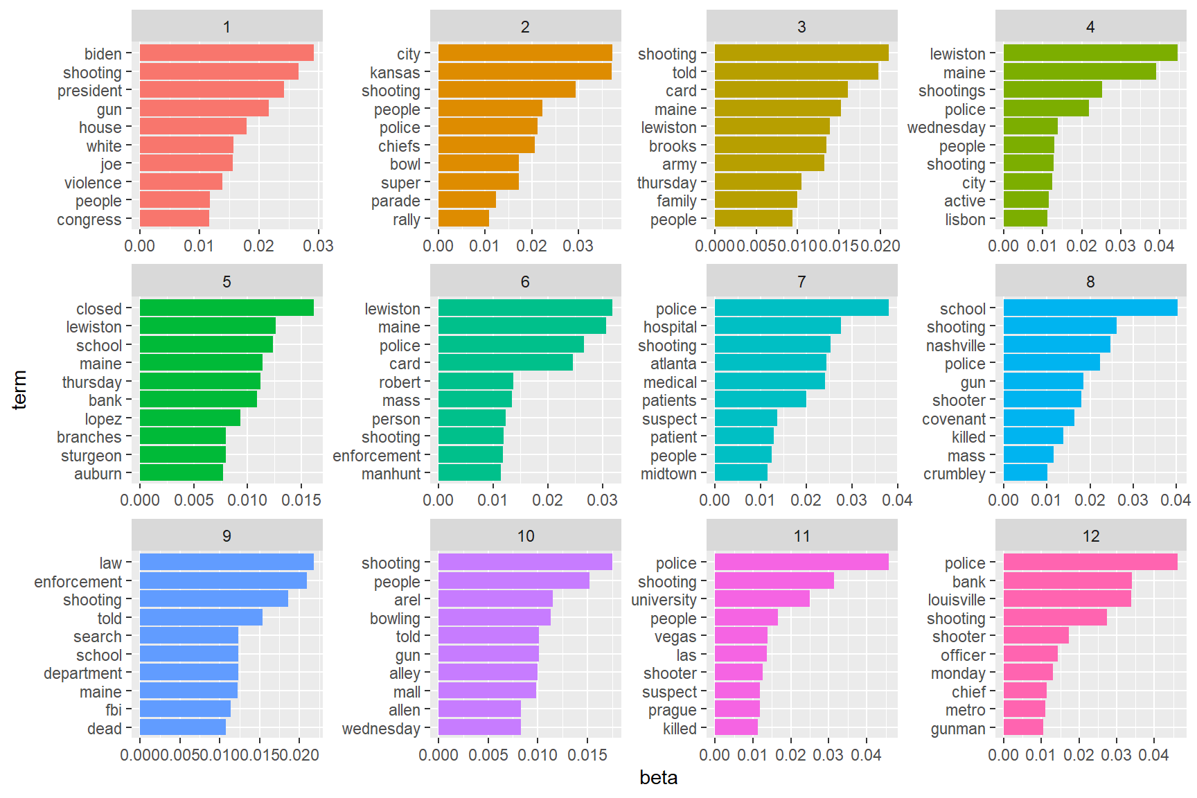
model1TopicsYou might have noticed the issue with the reverse naming of document and word. For some reason there happens a switch in the LDA() step, that I was unable to diagnose, so this is my shoddy workaround. Now that we have the model we can look how certain terms are present in the models 12 topics. Remember that the topics were set by the model itself and not by us. Therefor we can evaluate if the topic are sensible to our human preferences.
shootingTopTerms <- model1Topics %>%
  group_by(topic) %>%
  slice_max(beta, n = 10) %>%
  ungroup() %>%
  arrange(topic, -beta)

shootingTopTerms %>%
  mutate(term = reorder_within(term, beta, topic)) %>%
  ggplot(aes(beta, term, fill = factor(topic))) +
  geom_col(show.legend = FALSE) +
  facet_wrap(~ topic, scales = "free") +
  scale_y_reordered()
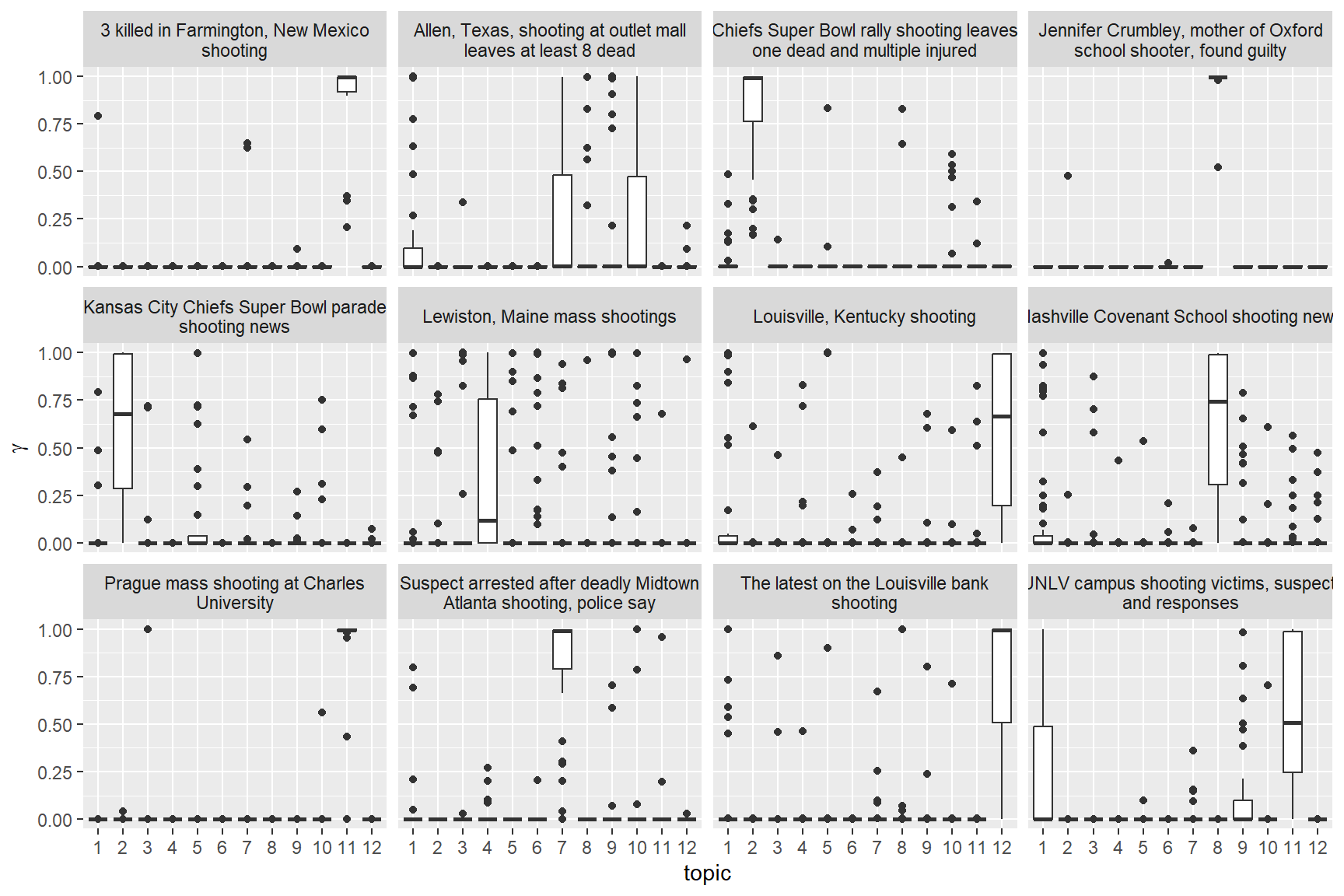
We are mostly interested in plot nr. 11 that is showing the language used during the reporting on the Prague mass shooting. To my sensibilities the graph make sense and so I will continue with the analysis. To determine whether the Prague shooting was a routing reporting experience for the writers at CNN we can look whether the articles themselves are significantly different. For that purpose we will separate the individual articles from their Events and look how many the model can correctly allocate to the correct topic.
model1Gamma <- tidytext::tidy(model1, matrix = "gamma")

model1Gamma
separatedGamma <- model1Gamma %>%
separate(document, c("Event", "Headline"), sep = "_", convert = TRUE)
separatedGammaseparatedGamma %>%
mutate(title = reorder(Event, gamma * topic)) %>%
ggplot(aes(factor(topic), gamma)) +
geom_boxplot() +
facet_wrap(~ Event) +
labs(x = "topic", y = expression(gamma))
Looking at the graph we can clearly see that there are 3 Events with significantly lower mis-attribution of articles/headlines they are: The Farmington New Mexico shooting, the judgment against Jennifer Crumbley and the Prague university shooting.
Conclusion
The uniqueness of these three events is understandable; the shooting in Farmington was unique in the age of its victims (73-97) and the method of its perpetrator, the case against Jenifer Crumbley was poised to set a precedent in the USA (by now it has set it already) and the shooting in Prague has shown the danger of exporting the motivations and conditions of mass shooting from the USA into other countries with similar cultural contexts.